Interactive mapping of biogeographical regions from species distributions

The original implementation is described in:
Edler, D., Guedes, T., Zizka, A. Rosvall, M. Antonelli, A. (2017) Infomap Bioregions: Interactive mapping of biogeographical regions from species distributions. Systematic Biology 66(2):197–204, doi: 10.1093/sysbio/syw087
It is based on the method described in:
Vilhena, D., Antonelli, A. (2015) A network approach for identifying and delimiting biogeographical regions. Nature communications 6, 6848
The original clustering algorithm is described in:
Rosvall, M. Bergstrom, C. (2008) Maps of information flow reveal community structure in complex networks, PNAS 105, 1118
If you are using Infomap Bioregions in one of your research articles or otherwise want to refer to it, please cite the relevant publication above or use the following format:
D. Edler, T. Guedes, A. Zizka, M. Rosvall, and A. Antonelli, Infomap Bioregions, available online at https://bioregions.mapequation.org.
If you have any questions, suggestions or issues regarding the software, please add them to GitHub issues.

As species distribution input, Infomap Bioregions supports both point occurrence data and species range maps.
Point occurrences are specified in a text file with either comma-separated (CSV) or tab-separated (TSV) values. The application requires a header with the column names, and the user must identify which columns that should be parsed as name, latitude and longitude, respectively.
Name, Lat, Long
Sp1, -5.61, -53.43
Sp1, -8.22, -48.90
Sp2, -8.17, -50.06
Range maps are specified in the shapefile format, which includes multiple files: a .shp file for species range polygons, a .dbf file for the attributes of each range polygon and, optionally, a .prj file for projection information. As for point occurrence data, the user must identify which attribute to parse as the name of the species.
Infomap Bioregions also supports loading a phylogenetic tree to show a phylogram and how it maps to the bioregions, if the names in the tree match with the names in the species distribution data. It supports the NEXUS and Newick tree format.
(A:0.1,B:0.2,(C:0.3,D:0.4):0.5);
The above example represents this tree:


Infomap Bioregions bins the species records into quadratic grid cells. To allow for adaptive spatial resolution, each grid cell can be recursively subdivided into four cells. The adaptive binning generates a so-called quadtree with subdivided grid cells that satisfy the following user-specified criteria, with decreasing priority from 1 to 3:
For point occurrence data, these criteria make the adaptive binning straightforward. For range maps, the application first adds a species record to each cell of minimum size that intersects with the corresponding species range polygon, and then proceeds with the adaptive binning to satisfy the user-specified criteria.

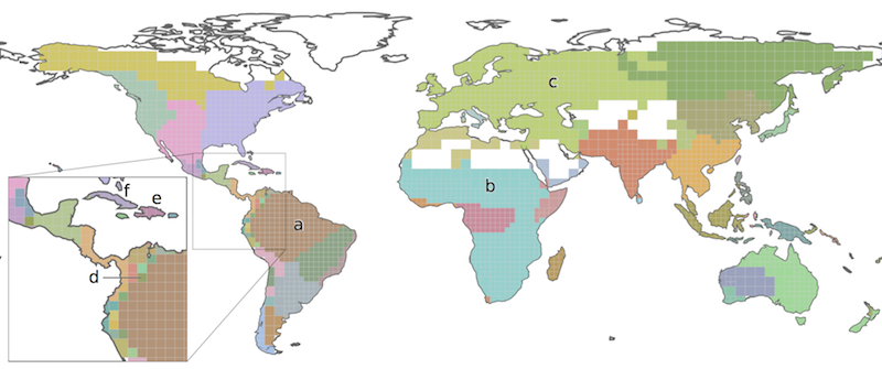
Infomap Bioregions generates a bipartite network of species and grid cells. Each species is connected by an unweighted link to each grid cell in which it is present. The network is clustered with the Infomap clustering algorithm for bipartite networks. In that process, the geographical grid cells are merged into different clusters which become the resulting bioregions.

The bipartite network of species and geographical grid cells is clustered with the Infomap clustering algorithm to find an optimal partition of the geographical space with respect to the map equation.

Each cluster of grid cells is given a unique color and forms a bioregion.

The bioregions can be exported both as a visual map (.png or .svg) and as structured data for further analysis (in the GeoJSON or shapefile format).
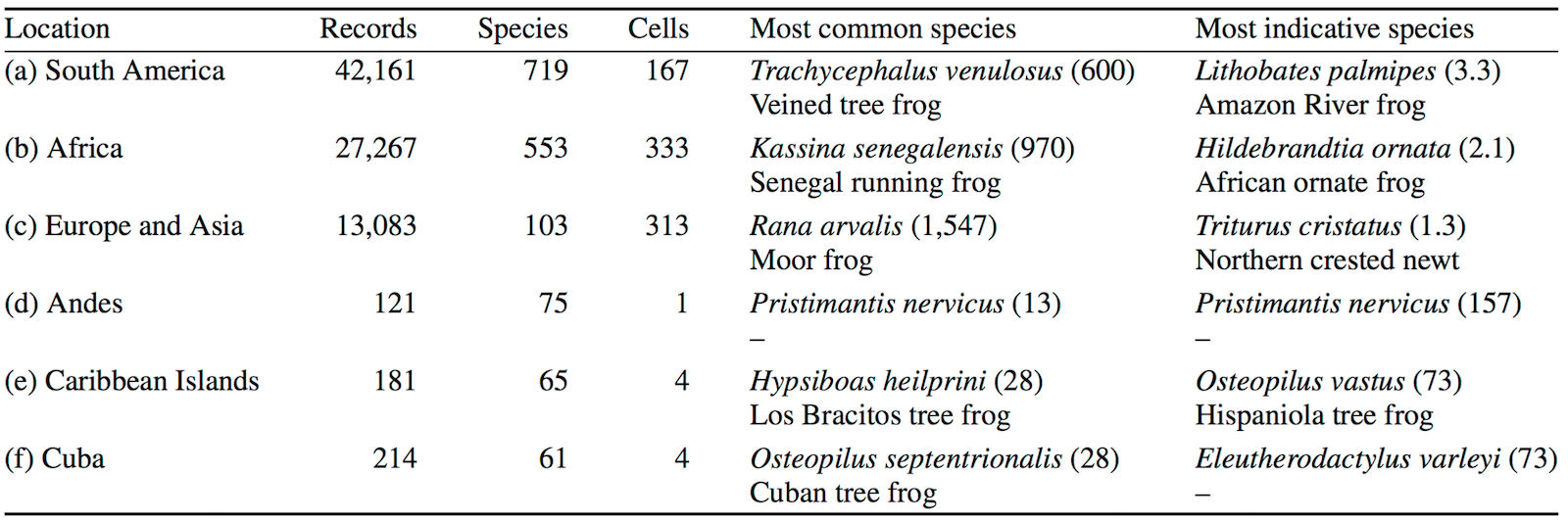
The application also identifies the most common and the most indicative species in each grid cell and bioregion, and shows the results as an interactive map together with supporting tables with information about the bioregions. These tables can be exported in the .csv format.